
Default labels are slow and coarse: waiting a year to find out who defaulted, then collapsing every borrower into default or not-default. This article shows how Markov Chains turn that binary label into a continuous probability of default, and what that buys in practice: risk models that perform better on small data, and portfolio comparisons that finally line up.
Why Are Default Labels Hard to Get Right?
Time-Lagged Default Labeling
The assignment of risk model labels can be significantly delayed depending on the definition of default. For instance, if a default is defined as 60 days past due (DPD) within a one-year period, a full year of observation is required to accurately assign these labels. This extended timeframe poses challenges for timely risk modeling. Even when employing interim weak labels to circumvent the one-year wait, the identification of a 60 DPD event remains delayed, as the observation period for confirming such defaults is inherently protracted, impacting the responsiveness of risk assessment and portfolio analysis.
Inconsistent Data Quality
Data consistency remains a critical challenge in developing machine learning models and data science applications. In an ideal scenario, highly consistent data (see the right-hand side of the charts below) enables models to perform effectively with smaller datasets. However, real-world data frequently exhibits variability and inconsistencies, requiring significantly larger datasets to ensure reliable model performance.
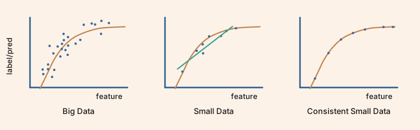
Data Consistency in Risk Model

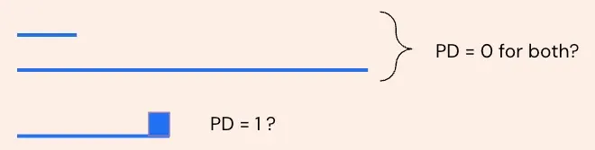
Financial risk models commonly use binary labels, defining default as an event like 60 DPD within one year. This binary approach (default or non-default) simplifies credit risk assessment and aligns with industry standards. However, it oversimplifies complex risk profiles, ignoring nuances (e.g., 59 DPD vs. 60 DPD) and requires a full year’s observation, delaying labeling. Markov Chains address this by converting binary labels into continuous labels, modeling risk through probabilistic state transitions for a more dynamic and accurate representation of borrower risk, enhancing risk models and portfolio analysis.
Data Consistency in Business Terms
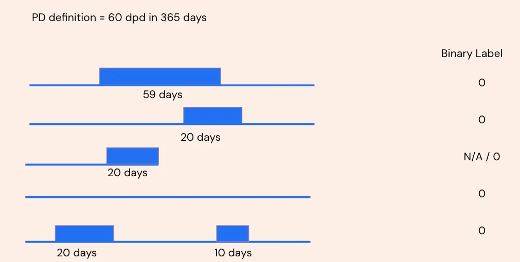
The chart above depicts repayment behavior over time (days), represented by two states: State 0 (current, no past due) and State 1 (delinquent, any past due status). In this binary risk model, all accounts not reaching 60 DPD are assigned a “non-default” (0) label, irrespective of delinquency severity. This leads to counterintuitive outcomes, such as accounts at 59 DPD or 20 DPD being labeled identically to those at 0 DPD, despite varying risk levels. Such oversimplification compromises accurate risk assessment, underscoring the value of Markov Chains for more granular, continuous labeling to better reflect credit risk dynamics.
How Does the Markov Label Get Computed?
Markov Chains turn a binary default label into a probability of default between 0 and 1.
Markov Chains transform binary labels into continuous values between 0 and 1, representing the probability of default based on a specified number of days past due (e.g., 60 DPD) within a given timeframe (e.g., one year).
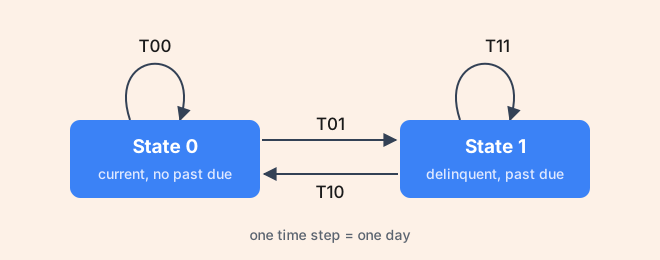
Two essential components must be defined: states and time-step size. The model specifies two states, State 0 (current, no past due) and State 1 (delinquent, any past due status), with a daily time step. Each account moves between the states day by day, with four transition probabilities:
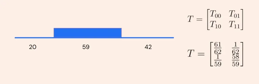
This section outlines the implementation process, focusing on practical steps without exploring Markov Chain theory in depth.
Per the chart above, the repayment history spans 20, 59, and 42 days. Of these, 20 + 42 days are in State 0, with 1 day transitioning from State 0 to State 1, so T01=1/(20+42) and T00=1−T01. Additionally, 59 days are in State 1, with 1 day transitioning from State 1 to State 0, so T10=1/59 and T11=1−T10. In code, each account’s repayment history becomes one 2x2 matrix:
# one row per state: [stay, leave] (State 0 = current, State 1 = past due)
T = np.array(
    [
        [1 - t01, t01],  # T00, T01: a day in state 0, next day
        [t10, 1 - t10],  # T10, T11: a day in state 1, next day
    ]
)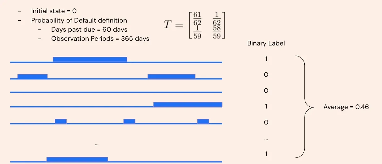
Using the transition matrix, multiple scenarios can be simulated based on a defined default threshold, generating a binary label for each scenario. For instance, simulating one year of repayment behavior, an account exceeding 60 DPD is labeled as 1 (default), otherwise 0 (non-default). By repeating this simulation and averaging the outcomes, a continuous Markov label is derived, literally representing the probability of default:
state = 0
dpd = 0
for _ in range(observation_days):
    state = rng.choice(2, p=T[state])
    dpd = dpd + 1 if state == 1 else 0
    if dpd >= dpd_threshold:  # e.g. 60
        break
label = dpd >= dpd_threshold
Note
The walkthrough above skips the algorithm’s full time complexity. In practice the simulation vectorizes; that is outside this article’s scope.
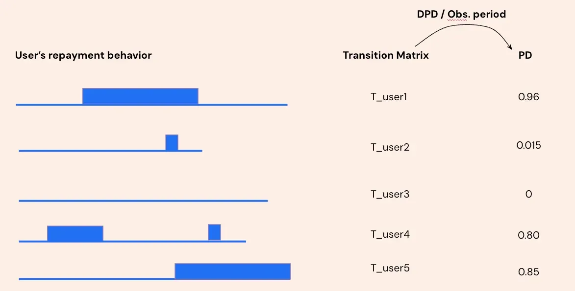
In conclusion, an individual account’s repayment behavior can be converted into a transition matrix, which is then used to derive a probability of default label based on a defined DPD threshold and observation period.
From Theory to Practice: Markov Chains in FinTech
Drawing from my real-world experience implementing Markov Chains in FinTech, I have observed significant advantages for both risk modeling and portfolio analysis, as detailed below.
Risk Model
Tip
Below 100,000 samples, Markov labels lifted the Gini coefficient by over 10% versus binary labels.
- Enhanced Performance with Limited Data: Markov Chains substantially improve model performance when sample sizes are below 100,000, achieving a Gini coefficient increase of over 10% in early stages with small datasets and short observation periods.
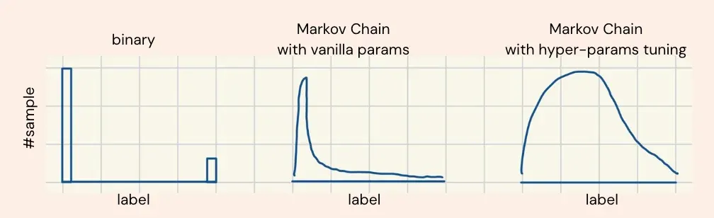
- Hyperparameter Optimization for Large Datasets: Markov Chains introduce additional hyperparameters, such as days past due (DPD) and observation period, enabling fine-tuning to maximize model performance. Incorporating Laplace smoothing as a prior adds further tunable parameters, as illustrated in the image below. This hyperparameter optimization yields a Gini coefficient improvement of approximately 2.5% compared to binary labeling, even with datasets of around one million samples.

Portfolio Analysis
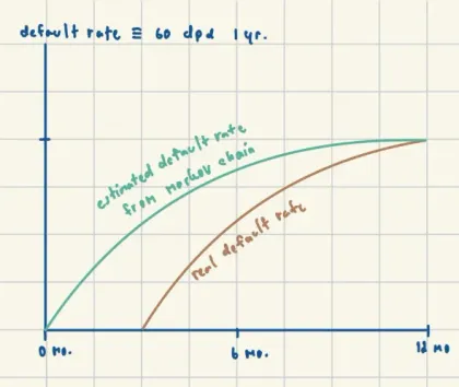
- Accelerated Feedback as a Leading Indicator: Markov Chain risk labels serve as a leading indicator for risk metrics, providing faster feedback compared to traditional binary-derived metrics like default rates, as demonstrated in the image below.
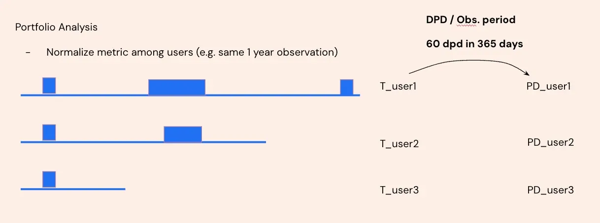
- Normalization Across Observation Periods: Markov Chain risk labels enable normalization of user risk profiles across varying observation periods. For instance, comparing users with a 6-month history to those with a 3-year history can be challenging; however, Markov Chain risk labels standardize both to a common period (e.g., one year), facilitating an equitable, apples-to-apples comparison.
Markov Chains offer a powerful approach to enhance risk modeling and portfolio analysis in FinTech, delivering improved model performance, accelerated feedback, and normalized risk comparisons across diverse datasets. By transforming binary labels into continuous probabilities, they enable more accurate and actionable insights for financial practitioners. However, this methodology introduces trade-offs, including increased implementation complexity and reduced explainability, which practitioners must weigh. Nevertheless, adopting Markov Chains can drive more robust risk management strategies, empowering organizations to navigate complex financial landscapes with greater precision.